Tensorflow二

上一节讲了tensorflow简单的运算，这节用简单的线性模型感受一下tensorflow和机器学习的一般操作。本章节只讲tensorflow的用法，如果对线性模型不了解的可以自行查阅，或者等博主有空写个专题（涉及基本原理和公式的推导）。
讲两个模型，线性回归(numpy造一些数据)，逻辑回归（mnist数据集）

从线性回归开始

线性回归：找到一组参数，作用于样本的属性，使其预测结果与真实结果接近（自行理解接近）

用tensorflow求解参数W，b，拟合样本数据，并matplotlib展示

直接上代码吧

import tensorflow as tf
import numpy
import matplotlib.pyplot as plt

#params:设定超参数
learning_rate = 0.01
training_epochs = 1001

train_x = numpy.asarray([3.3,4.4,5.5,6.71,6.93,4.168,9.779,6.182,7.59,2.167,
                         7.042,10.791,5.313,7.997,5.654,9.27,3.1])
train_y = numpy.asarray([1.7,2.76,2.09,3.19,1.694,1.573,3.366,2.596,2.53,1.221,
                         2.827,3.465,1.65,2.904,2.42,2.94,1.3])


n_samples = train_x.shape[0]
#需要注意的是当train_x是向量形式时，他的表示方式。
print(train_x.shape)
#线性回归，找到一组参数，作用于x,使其接近于y
X = tf.placeholder('float')
Y = tf.placeholder('float')

#w参数一般会给一个非0的初始值,取名为weights,b为偏移
#不加说明的命名规范，矩阵用大写
W = tf.Variable(numpy.random.randn(),name='weights')
b = tf.Variable(numpy.random.randn(),name= 'bias')

#预测结果
pred = tf.add(tf.multiply(X,W),b)

#定义损失函数，一般线性回归用均方误差即可（别告诉我你不知道分母为什么）
cost = tf.reduce_sum(tf.pow(pred-Y,2))/(2*n_samples)
#定义优化器,这里选择随机梯度下降
optimizer =  tf.train.GradientDescentOptimizer(learning_rate).minimize(cost)

#初始化定义的变量
init = tf.global_variables_initializer()
with tf.Session() as sess:
    sess.run(init)
    #训练模型
    for epoch in range(training_epochs):
        for (x,y) in zip(train_x,train_y):
            sess.run(optimizer,feed_dict={X:x,Y:y})
        if epoch % 50 == 0:
            c = sess.run(cost,feed_dict={X:train_x,Y:train_y})
            #每50次看一下训练的效果
            print("Epoch:", '%04d' % (epoch), "cost=", "{:.9f}".format(c),
                  "W=", sess.run(W), "b=", sess.run(b))
    print("Optimization Finished!")
    training_cost = sess.run(cost, feed_dict={X: train_x, Y: train_y})
    print("Training cost=", training_cost, "W=", sess.run(W), "b=", sess.run(b), '\n')

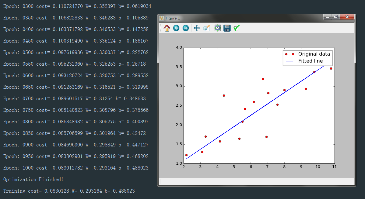
    #画图，这里的'ro'r指的red,o指的是散点图
    plt.plot(train_x, train_y, 'ro', label='Original data')#加0变成散点图
    plt.plot(train_x, sess.run(W) * train_x + sess.run(b), label='Fitted line')
    #legend显示label
    plt.legend()
    plt.show()

程序截图

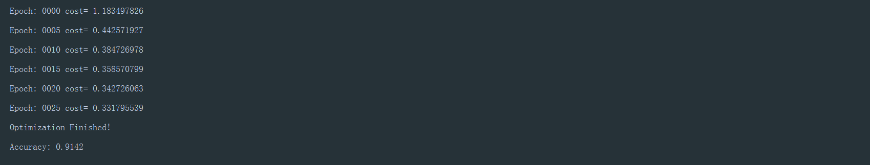
逻辑回归

逻辑回归：在线性回归的基础上，用sigmoid函数对值域进行控制（0，1）之间，逻辑回归处理二分类问题，这里用mnist数据集，用softmax函数代替，损失函数用交叉熵代替。（不明白交叉熵就等我更新喽）

tensorflow as tf

from tensorflow.examples.tutorials.mnist import  input_data

mnist = input_data.read_data_sets('/tmp/data/',one_hot=True)

#Params:
learning_rate = 0.01
training_epochs = 26
batch_size = 100

x = tf.placeholder(tf.float32,[None,784])
y = tf.placeholder(tf.float32,[None,10])

W = tf.Variable(tf.zeros([784,10]))
b = tf.Variable(tf.zeros([10]))
#预测结果
#matmul表示矩阵乘法
pred = tf.nn.softmax(tf.matmul(x,W)+b)
#损失函数采用交叉熵
cost = tf.reduce_mean(-tf.reduce_sum(y*tf.log(pred),reduction_indices=1))
optimizer = tf.train.GradientDescentOptimizer(learning_rate).minimize(cost)
init = tf.global_variables_initializer()
with tf.Session() as sess:
    sess.run(init)
    for epoch in range(training_epochs):
        avg_cost = 0
        total_batch = mnist.train.num_examples // batch_size
        for i in range(total_batch):
            batch_x,batch_y = mnist.train.next_batch(batch_size)
            _,c = sess.run([optimizer,cost],feed_dict={x:batch_x,y:batch_y})
            avg_cost += c/total_batch
        if epoch%5==0:
            print("Epoch:", '%04d' % (epoch), "cost=", "{:.9f}".format(avg_cost))
    print("Optimization Finished!")
    correct_prediction = tf.equal(tf.argmax(pred,1),tf.argmax(y,1))
    #求平均值，如果不明白可以单独写一个demo去测试tf.cast(),tf.reduce_man()方法。
    #需要注意的是这里的correct_prediction以及accuracy是 op ,必须放到会话中去运行。
    accuracy = tf.reduce_mean(tf.cast(correct_prediction,tf.float32))
    # print('correct_prediction',sess.run(correct_prediction,{x: mnist.test.images, y: mnist.test.labels}))
    print("Accuracy:", accuracy.eval({x: mnist.test.images, y: mnist.test.labels}))