GAN

有关生成模型

对于非监督学习，生成模型指的是找到一个模型生成的分布跟数据的真实分布越接近越好。在接近的同时如果能够抓住真实数据集的重要特征，并能保持高的清晰度(这里指的是图片，当然也有文本的)，可以说这算是一个好的生成模型。举例说，给定一个人脸数据集，训练模型后，测试生成一张人脸照片，并且这张照片好似来自于这个数据集，并且颜色纹理轮廓都较为清晰。

生成模型
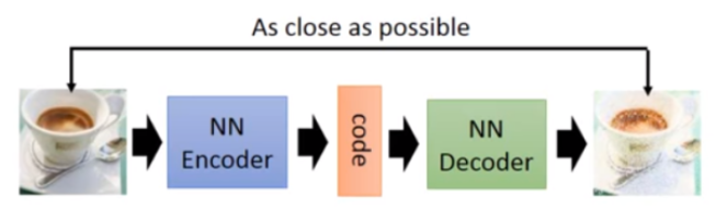
auto-encoder

针对图像训练：开始训练一个encoder，转化input成code，再训练一个 decoder，把code转为image。训练完结束只需要一个decoder，随机给一个code，自动生成一张图片。

VAE
先占标题

Idea of GAN
在讲述GANS网络之前，先简单谈谈自己的理解，为什么要想出GAN?GAN的优点在哪？GAN解决了什么样的问题？
分析如下：
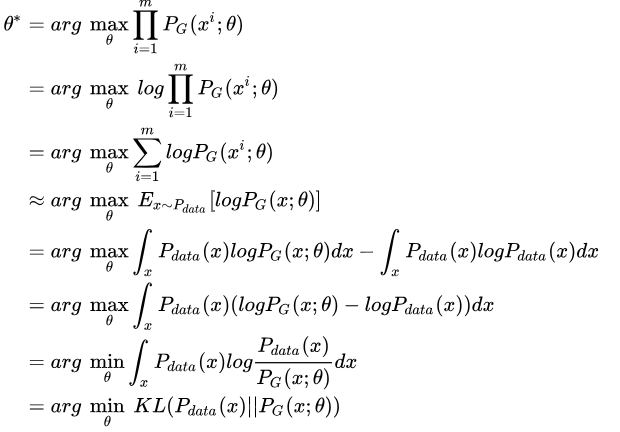
是否直接训练一个generator，通过极大似然来求解最佳参数呢？假设在真实分布中取出一些数据$x^1,x^2,\ldots,x^m$,生成模型分布为$P_G(X^i;\theta)$，那么这些数据的似然为$L=\prod_{i=1}^m P_G(x^i;\theta)$，最大化该似然函数等价于让generator生成真实图片的概率最大。求解该似然函数
关于减号后面的项和$\theta$无关，添上之后可以理解为等价。最后经过转换可以得到KL-divergence形式，通过最大似然最终可以得到两个分布之间的KL-divergence，那么问题来了$P_G(x;\theta)$计算相当困难，尤其是G是神经网络。接着就是GAN的贡献了。 $V(G,D)=E_{x-Pdata}logD(x)+E_{x-PG}log(1-D(X))$ (需要注意的是，此处给出的式子是等价后的式子，没有noise z)通过一个额外的Discriminator来做分类。主要思想就是：Discriminator 判别数据是来自Pdata，还是来自于Pg。当Pg生成的数据较好的时候，Discriminator已经无法正确分辨，此时accuarcy接近50%。
接下里如何训练呢？

train GANS
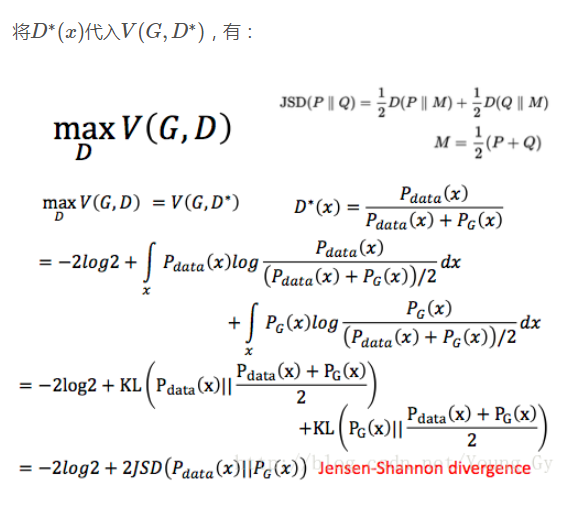
整个策略是，G0的参数先随机生成，固定G，求Max V(G,D)的D*，然后固定D*，min V(G,D*)，是一个交替训练的过程。
有关D的训练推导比较简单，求期望转化为积分的形式，再对积分号里面的内容进行求导求最大值。
$V(G,D)=\int\left[P_{data}logD(x)+P_G log(1-D(x))\right]dx$ $D*=arg max_D P_{data(x)}logD(X)+P_{G(x)} log(1-Dx)$ $D*(x)=\frac{P_{data (x)}}{P_{data (x)}+P_G (x)}$
每个D*(x)对应的V(G,D)实际上等价于两个分布之间的差距(手打公式太累了)。
有关G的训练更简单了min V(G0,D*)，最小化分布之间的差异，即固定D*，优化G。
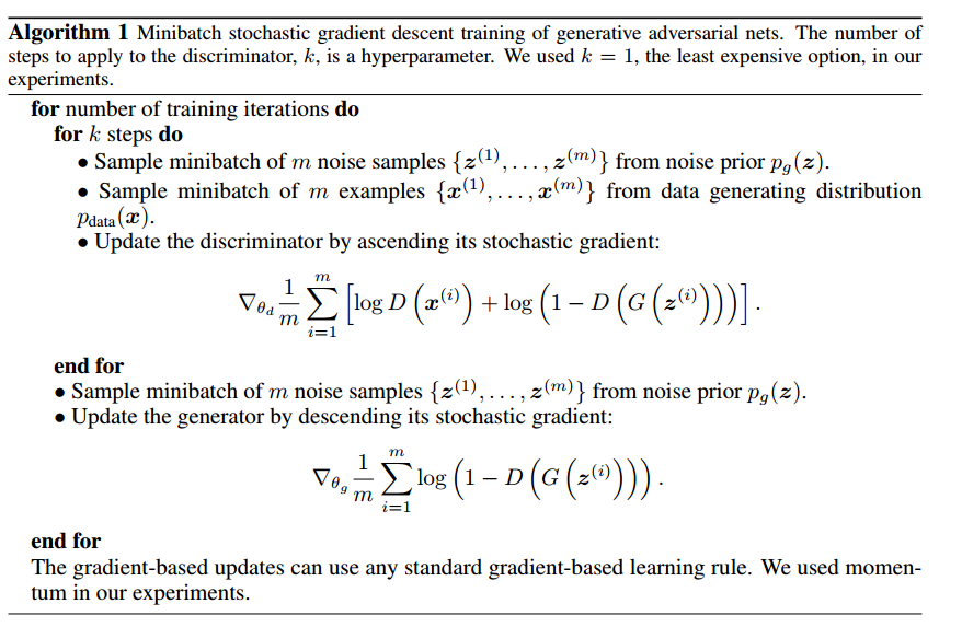
贴上论文的训练算法：

Pipline

回过头再来看看GAN做了什么的事情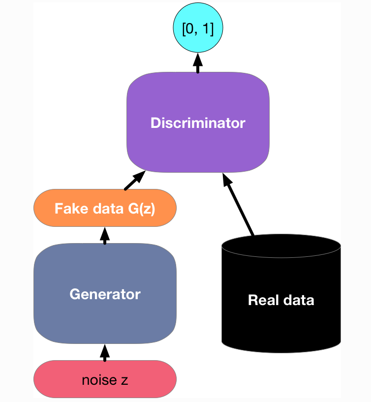

问题

G的更新优化不一定朝着最小的方向。

从图中可以看得比较明显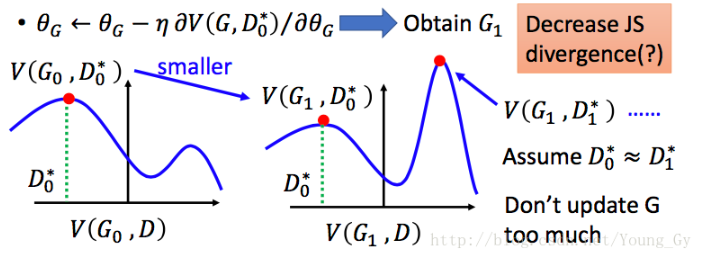

根据训练algorithm交替训练，可能在 D0* 的位置取到 $maxV(G0,D0)=V(G0,D0*)$，然后更新G0为G1，可能$V(G1,D0*) < V(G0，D0*)$了，但是不能保证找到一个新的D1* 使得$V(G1,D1*)>V(G0,D0*)$关于这一点理解的不是很好。

有关G的目标函数问题

log(1-D(x)) 作为loss function，在D(x)接近0，梯度很小，在训练初期变得很缓慢。而-log(D(x))也是递减，优势在于D(x)在接近0时，梯度很大，有利于训练，在D(x)越来越大后，梯度减小符合实际需求。

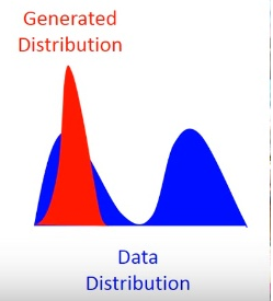
在训练过程中max V(G,D)=0

说明JS-divergence 一直是log2，Pdata和Pg没有交集。原因可能是因为:无法真正计算期望和积分，只能随机sample，导致过拟合，D过于强大，将两个数据集完全区别开。
办法：加noise，并且随着训练的时间，减少noise，这是由于loss function带来的缺陷。

model collapse

造成这个现象来源于KL-divergence里面的两个分布写反了。为了防止造成无穷大，只学习Pdata分布有的。

代码

#encoding=utf-8
from __future__ import print_function
import mxnet as mx
from mxnet import gluon,autograd,nd
from mxnet.gluon import nn
from matplotlib import pyplot as plt
## generating data
ctx = mx.cpu()
X = nd.random_normal(shape=(1000,2))
A = nd.array([[1,2],[-0.1,0.5]])
b = nd.array([1,2])
X = nd.dot(X,A)+b
Y = nd.ones(shape=(1000,1))

batch_size = 4
real_data = mx.io.NDArrayIter(X,Y,batch_size,shuffle=True)



## define the networks
G = nn.Sequential()
with G.name_scope():
    G.add(nn.Dense(2))
D = nn.Sequential()
with D.name_scope():
    D.add(nn.Dense(5,activation='tanh'))
    D.add(nn.Dense(3,activation='tanh'))
    D.add(nn.Dense(2))

## loss
loss = gluon.loss.SoftmaxCrossEntropyLoss()

## initialize the networks
G.initialize(mx.init.Normal(0.02),ctx=ctx)
D.initialize(mx.init.Normal(0.02),ctx=ctx)

trainnerG = gluon.Trainer(G.collect_params(),'adam',{'learning_rate':0.01})
trainnerD = gluon.Trainer(D.collect_params(),'adam',{'learning_rate':0.05})
## labels
real_label =mx.nd.ones((batch_size,),ctx=ctx)
fake_label =mx.nd.zeros((batch_size,),ctx=ctx)
# print('real_label shape',real_label.shape)
# print('fake_label shape',fake_label.shape)
#about Accuracy u can find in source code
metric = mx.metric.Accuracy()

#have a habit of setting a stamp
from datetime import datetime
import os
import time
stamp = datetime.now().strftime('%Y_%m_%d_%H_%m')
for epoch in range(9):
    tic =time.time()
    #Does it needs to reset
    real_data.reset()
    for i,batch in enumerate(real_data):
        data = batch.data[0].as_in_context(ctx)
        noise = nd.random_normal(shape=(batch_size,2),ctx=ctx)
        with autograd.record():
            r_output = D(data)
            err_r = loss(r_output,real_label)
            fake = G(noise)
            f_output = D(fake.detach())
            err_f = loss(f_output,fake_label)
            errD = err_r + err_f
            errD.backward()
        trainnerD.step(batch_size)
        # print('r_output shape',r_output.shape)
        # print('f_output shape',f_output.shape)
        metric.update([real_label,],[r_output,])
        metric.update([fake_label,],[f_output,])
        with autograd.record():
            output = D(fake)
            errG = loss(output,real_label)
            errG.backward()
        trainnerG.step(batch_size)
    name,acc = metric.get()
    metric.reset()
    print('\ntraining acc at epoch {0}:{1}={2}'.format(epoch,name,acc))
    print('time:{0}'.format(time.time()-tic))
    noise = nd.random_normal(shape=(100,2),ctx=ctx)
    fake = G(noise)
    plt.scatter(X[:,0].asnumpy(),X[:,1].asnumpy())
    plt.scatter(fake[:,0].asnumpy(),fake[:,1].asnumpy())
    plt.show()

结果

Reference

https://gluon.mxnet.io/chapter14_generative-adversarial-networks/gan-intro.html
https://zhuanlan.zhihu.com/p/27295635
paper of Generative Adversarial Nets